Modeling flammability limits in hydrogen-air mixtures using Mathematica
This post demonstrates how to use Mathematica to calculate and visualize the 3 flammability limits that occur in hydrogen-air mixtures. The implementation calculates reaction durations across various pressure and temperature conditions to identify these critical boundaries.
1 Equations of hydrogen combustion
The values of constants and kinetic equations are taken from the author of the KINET program A. V. Abramenkov (Lomonosov MSU, Moscow).
H2 + O2 = OH + OH,      k = 1.48 e + 10, 161.080
OH + OH = H2 + O2,      k = 4.6 e + 08, 85.600
OH + H2 = H2O + H,      k = 2 e + 10, 21.760
H2O + H = OH + H2,      k = 8.5 e + 10, 86.400
H + O2 = OH + O,        k = 2.5 e + 11, 71.760
OH + O = H + O2,        k = 2.55 e + 10, 1.570
O + H2 = OH + H,        k = 5.66 e + 09, 36.610, 1.00
OH + H = O + H2,        k = 2.46 e + 09, 29.290, 1.00
O + H2O = OH + OH,      k = 7 e + 10, 77.610
OH + OH = O + H2O,      k = 6.5 e + 09, 4.810
H + H + M = H2 + M,     k = 6.5 e + 08
H2 + M = H + H + M,     k = 6.71 e + 12, 428.860, -1.00
O + O + M = O2 + M,     k = 6.5 e + 08
O2 + M = O + O + M,     k = 2.35 e + 13, 500.820, -1.00
H + OH + M = H2O + M,   k = 1.69 e + 12, , -2.00
H2O + M = H + OH + M,   k = 2.5 e + 13, 442.670
OH + OH + M = H2O2 + M, k = 8.75 e + 08, -21.610
H2O2 + M = OH + OH + M, k = 1.2 e + 14, 191.210
OH + O + M = HO2 + M,   k = 4.75 e + 10
HO2 + M = OH + O + M,   k = 1 e + 12, 280.330
H + O2 + M = HO2 + M,   k = 2.7 e + 09, -6.020
HO2 + M = H + O2 + M,   k = 2.25 e + 12, 194.140
HO2 + H2 = H2O2 + H,    k = 7.25 e + 08, 82.840
H2O2 + H = HO2 + H2,    k = 1.55 e + 09, 16.740
HO2 + H2 = H2O + OH,    k = 1.15 e + 08, 99.580
H2O + OH = HO2 + H2,    k = 2.76 e + 07, 232.630, 0.50
HO2 + H2O = H2O2 + OH,  k = 2.5 e + 10, 135.980
H2O2 + OH = HO2 + H2O,  k = 1.15 e + 10, 7.410
HO2 + HO2 = H2O2 + O2,  k = 3 e + 09
H2O2 + O2 = HO2 + HO2,  k = 2.16 e + 09, 172.380, 0.50
H + HO2 = OH + OH,      k = 2 e + 11, 7.470
OH + OH = H + HO2,      k = 1.15 e + 10, 168.620
H + HO2 = H2O + O,      k = 1.4 e + 10, 8.740
H2O + O = H + HO2,      k = 5.5 e + 09, 242.670
H + HO2 = H2 + O2,      k = 4 e + 10, 2.510
H2 + O2 = H + HO2,      k = 5.5 e + 10, 241.840
O + HO2 = OH + O2,      k = 3.5 e + 10
OH + O2 = O + HO2,      k = 3.5 e + 10, 236.400
H + H2O2 = H2O + OH,    k = 1 e + 12, 44.770
H2O + OH = H + H2O2,    k = 1.15 e + 11, 333.460
O + H2O2 = OH + HO2,    k = 2.5 e + 10, 4.600
OH + HO2 = O + H2O2,    k = 3.8 e + 10, 50.210
H2 + O2 = H2O + O,      k = 5.5 e + 10, 228.030
H2O + O = H2 + O2,      k = 5.5 e + 10, 228.030
H2 + O2 + M = H2O2 + M, k = 3 e + 07, 83.260
H2O2 + M = H2 + O2 + M, k = 2.75 e + 10, 209.200
OH + M = O + H + M,     k = 2.5 e + 13, 432.210
O + H + M = OH + M,     k = 2.55 e + 10
HO2 + OH = H2O + O2,    k = 2 e + 10, 1.260
H2O + O2 = HO2 + OH,    k = 1.9 e + 11, 307.520, 0.50
H2 + O + M = H2O + M,   k = 2.75 e + 08
H2O + M = H2 + O + M,   k = 2.75 e + 14, 456.060
O + H2O + M = H2O2 + M, k = 7.5 e + 07, 50.210
H2O2 + M = O + H2O + M, k = 1.05 e + 12, 190.790
O + H2O2 = H2O + O2,    k = 1.3 e + 08, 112.970
H2O + O2 = O + H2O2,    k = 1.25 e + 09, 445.600
H2 + H2O2 = H2O + H2O,  k = 1.3 e + 10, 87.860
H2O + H2O = H2 + H2O2,  k = 3.5 e + 09, 460.240
H + HO2 + M = H2O2 + M, k = 1.9 e + 08, 5.230
H2O2 + M = H + HO2 + M, k = 1.5 e + 12, 380.740
Save the above data in a file named H2Burn.kin in the same directory as this notebook.
2 Extract data from file
We start by importing the reaction data from the file. The data is in a text format, so we use Import to read it:
str = Import["H2Burn.kin","Text"];Now we parse the reaction data. Each line contains a reaction equation and kinetic parameters:
lines = Replace[
  StringSplit[StringSplit[str,"\n"],RegularExpression[",\\s+"]],
  {{eq_,k_}:>{eq,k,0,0},{eq_,A_,Ea_}:>{eq,A,Ea,0}},
  1
];
Next, we extract the different components from our parsed data:
{reactionStrings, preExponential, activations, empirical} = Transpose@lines;The pre-exponential factors need to be converted to numerical values:
preExponential = Interpreter["Number"]@*StringDelete[RegularExpression["\\s+"]]/@StringTrim[preExponential,{"k = "}]/.Null->0;Similarly, we process the activation energies and empirical coefficients:
activations = 1000ToExpression/@activations/.Null->0;
empirical = ToExpression/@empirical;
We transform the reaction strings into rule-based format for easier processing:
rules = Rule@@@(StringSplit[#," + "]&/@StringSplit[reactionStrings," = "])/.Null->0;Finally, we extract all unique reagents from the reactions:
reagents = DeleteDuplicates@Flatten[List@@@rules];3 Transform data to system of equations
Now we’ll create a function that builds differential equations for each reagent. This function identifies reactions involving a specific reagent and computes its rate of change:
makeEq[reag_] := Module[{mask, factors, act, pre, emp, consts},
  mask = Map[Not@*FreeQ[reag], rules];
  factors = Cases[
    Pick[rules, mask],
    HoldPattern[r_->p_] :> Times@@(c[#][t]&/@r)(Count[reag]@p-Count[reag]@r)
  ];
  act = Pick[activations, mask];
  pre = Pick[preExponential, mask];
  emp = Pick[empirical, mask];
  consts = Replace[
    Transpose[{pre, act, emp}],
    {a_, e_, n_} :> a (T/298)^n Exp[-( e/(8.31 T))],
    1
  ];
  c[reag]'[t] == factors . consts
]
The rate constants follow the Arrhenius equation with temperature dependence.
Next, we build a complete system of differential equations for all reagents:
makeSys[init_, temp_] := Module[{eqs, inits, unconditioned, sys},
  eqs = makeEq/@reagents;
  unconditioned = Complement[reagents, First/@init];
  inits = init/.HoldPattern[r_->conc_]:>c[r][0]==conc;
  unconditioned = c[#][0]==0&/@unconditioned;

  sys = Join[eqs, inits, unconditioned]/.T->temp;
  sys = Select[sys, FreeQ[#,c["M"]'[t]==0.]&&FreeQ[#,c["M"][0]]&];
  sys = sys/.c["M"][t]->c["H2"][t]+c["N2"][t]+c["O2"][t];
  sys = sys/.c["N2"][_]->cN2;
  sys = sys/.True->Nothing;

  sys
]
Prepare the list of variables for which we’ll solve the system:
vars = DeleteDuplicates@DeleteCases[Map[c[#][t]&, reagents], c["M"][t]];Now we define the solver function that will integrate our system of ODEs:
sol[cH2_, cO2_, cN2_, T_, tmax_] :=
  Quiet@Module[{end = 1, sol1},
    sol1 = First @ NDSolve[
      makeSys[{"H2" -> cH2, "O2" -> cO2, "N2" -> cN2}, T],
      vars,
      {t, 0, tmax},
      Method -> {
        "EventLocator",
        "Event" -> {c["H2"][t] <= cH2 / 2 || c["O2"][t] <= cO2 / 2},
        "EventAction" :> Throw[end = t, "StopIntegration"]
      }
    ];
    {sol1, end}
  ]
4 Define measurable metrics
Now we define functions to characterize the flammability limits. First, a function to calculate reaction duration at a given pressure and temperature:
ClearAll[duration];
duration[p_, T_] := Module[{
  coeffs = {6.9797, 1.4657, 5.5140}10^-3,
  press
  },
  press = coeffs{p, p, p};
  Last@sol[Sequence@@press, T, 1]
]
Next, we define a function to calculate data points across a range of pressures and temperatures:
ClearAll[calculate];
calculate[{logPmin_, logPmax_}, {Tmin_, Tmax_}, grid_:10] :=
  Flatten[#, 1]& @ ParallelTable[
    {T, p, -Log10 @ duration[p, T]},
    {p, 10^Subdivide[logPmin, logPmax, grid]},
    {T, Subdivide[Tmin, Tmax, grid]}
  ];
5 Start parallel calculations and plot results
Now we run our calculation across a range of pressures (10^-3 to 10^3 atm) and temperatures (600 to 1000 K):
data = calculate[{-3, 3}, {600, 1000}, 10];Finally, we visualize the results as a contour plot showing the three distinct flammability limits:
ListContourPlot[
  data,
  ClippingStyle -> Automatic,
  ScalingFunctions -> {None, "Log10"},
  Epilog -> {
    Text[Style["1st limit", 20, White], Scaled[{.7, .3}]],
    Text[Style["2nd limit", 20, White], Scaled[{.7, .5}], Automatic, {1, 0.4}],
    Text[Style["3rd limit", 20, White], Scaled[{.5, .7}], Automatic, {1, -0.2}]
  },
  FrameLabel -> {"T, K", "p, atm"},
  PlotLegends -> Automatic,
  ColorFunction -> "TemperatureMap",
  PlotLabel -> "-lg [duration]"
]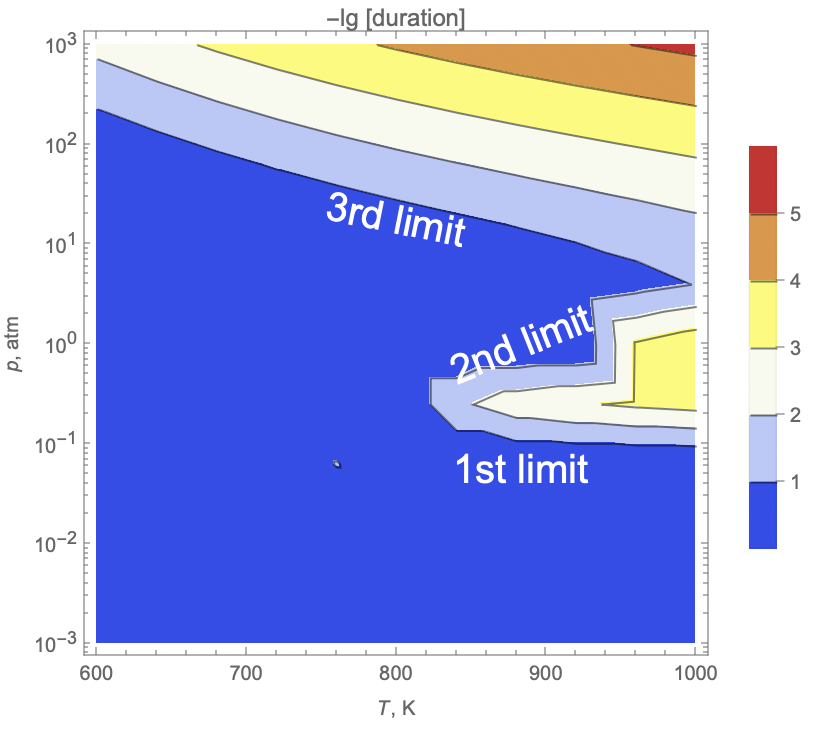
The resulting plot shows three distinct regions corresponding to the three flammability limits of hydrogen-air mixtures. These limits represent boundaries where combustion becomes sustainable or unsustainable based on mixture composition, pressure, and temperature conditions.