Calculation of pH titration curves in Mathematica

chemistry

mathematica

Published

November 5, 2018

Modified

April 30, 2025

Computer algebra systems are useful for solving chemical equilibria. Here, a simple example is presented: the titration of a dibasic acid with a strong base. The goal is to derive the pH titration curve and identify the equivalence points.

1 Chemical equilibria

A dibasic acid H_{2}Z dissociates in water in 2 steps:

\text{ H}_{2}\text{Z } + \text{ H}_{2}\text{O } \rightarrow \text{ H}_{3}O^{+} + \text{ HZ}^{-} \text{ HZ}^{-} + \text{ H}_{2}\text{O } \rightarrow \text{ H}_{3}O^{+} + \text{ Z}^{2 -}

During titration with a base like \text{NaOH}, the pH changes, and this can be modeled with a system of equations.

To model equilibria, we need to write three types of equations:

Equations of charge balance to ensure that the total charge in the solution is zero. \underset{\text{ positive ions}}{\underbrace{\left\lbrack H^{+} \right\rbrack + \left\lbrack \text{Na}^{+} \right\rbrack}} = \underset{\text{ negative ions}}{\underbrace{\left\lbrack \text{OH}^{-} \right\rbrack + \left\lbrack \text{HZ}^{-} \right\rbrack + 2\left\lbrack Z^{2 -} \right\rbrack}}
So-called mass balance equations which impose conservation of matter (ions and atoms of each type). \left\lbrack H_{2}Z \right\rbrack + \left\lbrack \text{HZ}^{-} \right\rbrack + \left\lbrack Z^{2 -} \right\rbrack = C - \left\lbrack \text{Na}^{+} \right\rbrack \left\lbrack \text{Na}^{+} \right\rbrack = \left( C - \left\lbrack \text{Na}^{+} \right\rbrack \right) \cdot \tau As we add base, the concentration of the acid decreases and the concentration of the conjugate base increases. The parameter \tau represents the degree of titration - when \tau = 1, we’ve added exactly enough base to neutralize the 1st proton in all acid molecules, and when \tau = 2, we’ve neutralized both protons.
All equilibrium constants for all reactions in the system. 10^{- pK_{a,1}} = \frac{\left\lbrack H^{+} \right\rbrack \cdot \left\lbrack \text{HZ}^{-} \right\rbrack}{\left\lbrack H_{2}Z \right\rbrack},\quad 10^{- pK_{a,2}} = \frac{\left\lbrack H^{+} \right\rbrack \cdot \left\lbrack Z^{2 -} \right\rbrack}{\left\lbrack \text{HZ}^{-} \right\rbrack} 10^{- pK_{w}} = \left\lbrack H^{+} \right\rbrack \cdot \left\lbrack \text{OH}^{-} \right\rbrack These equations represent stepwise acid constants K_{a,1}, K_{a,2} and water ion product K_{w} respectively.

In Mathematica, the system of equations can be represented as:

sys = {
  10^-pKa1 == (c["H+"] c["HZ-"])/c["H2Z"],
  10^-pKa2 == (c["H+"] c["Z2-"])/c["HZ-"],
  10^-pKw == c["H+"] c["OH-"],
  c["H2Z"] + c["HZ-"] + c["Z2-"] == conc - c["Na+"],
  c["Na+"] == (conc - c["Na+"]) τ,
  c["H+"] + c["Na+"] == c["OH-"] + c["HZ-"] + 2 c["Z2-"]
}

2 Solving the system

Mathematica can be used to solve the system of equations. We will use the Eliminate function to remove intermediate variables and get a single equation in terms of the hydrogen ion concentration c\left\lbrack \text{H+} \right\rbrack and our parameters.

elim = Eliminate[
  sys,
  {c["OH-"], c["H2Z"], c["HZ-"], c["Z2-"], c["Na+"]}
];

The Eliminate function removes intermediate variables, giving us a single equation in terms of c["H+"] and our parameters.

Now we can solve for the hydrogen ion concentration:

sol = Solve[elim, c["H+"]];

This gives us multiple possible solutions, but only one will be physically meaningful for our chemistry problem.

3 Substituting numerical values

To make our calculations concrete, we’ll use specific values for our constants.

Malic acid is a dibasic organic acid found in many fruits, with pKa values of 3.40 and 5.20. We’re modeling a solution with 1 molar concentration and titrating at 25°C.

consts = <|
  pKa1 -> 3.40,
  pKa2 -> 5.20, (* malic acid *)
  pKw -> 14.,    (* ion-product of water at 25 °C *)
  waterConc -> 55.35,         (* at 25 °C *)
  conc -> 1,                  (* acid concentration *)
  c["Na+"] -> τ               (* titrant *)
|>;

Near the equivalence point, the pH changes rapidly, requiring high precision calculations:

consts = SetPrecision[#, 100] & /@ consts;

Now we convert our hydrogen ion concentration to pH values:

solList = -Log10[c["H+"]]/.sol/.consts;

And select the physically meaningful solution:

f[τ_] = solList[[2]];

The function f[τ] now gives us the pH at any point during the titration.

4 Visualizing the titration curve

Let’s calculate points for our titration curve, sampling τ from 0 (no added base) to 2.5 (excess base):

titrationCurve = Table[{τ, f[τ]}, {τ, 0, 2.5, 1/1000}];

The derivative of the pH curve helps identify equivalence points, where we see sharp changes in pH:

df = f';

We’ll calculate this derivative curve as well:

diffCurve = Table[{τ, Chop@df[τ]}, {τ, 0, 2.5, 1/1000}];

Finally, we can plot both curves:

plot = ListLinePlot[
  {titrationCurve, diffCurve},
  PlotLegends -> {"pH(τ)", "dpH/dτ"},
  PlotRange -> {{0, 2.5}, {0, 14}},
  PlotTheme -> "Detailed",
  FrameLabel -> {"degree of titration τ"}
]

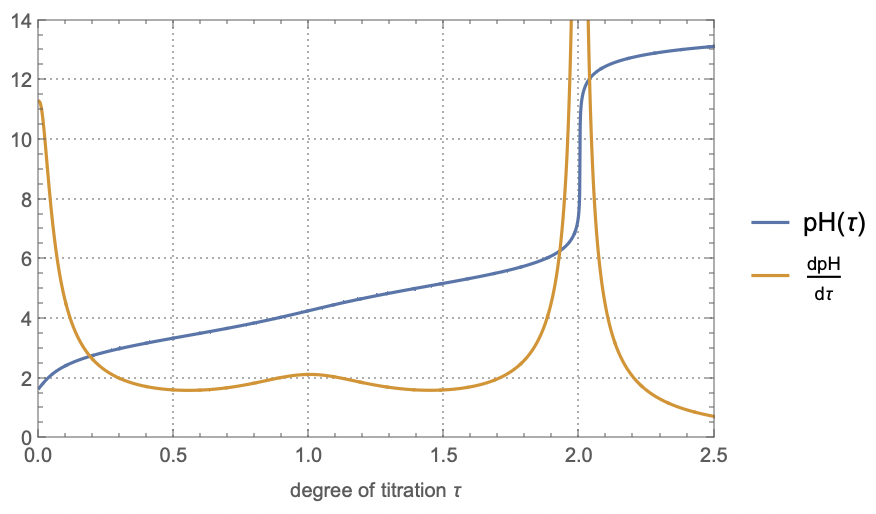
The differential curve (\frac{\mathrm{d}\text{pH}}{\mathrm{d}\tau}) shows peaks at these equivalence points. The buffer regions, where pH changes slowly, occur around \tau = 0.5 and \tau = 1.5.

These buffer regions correspond to solutions where the ratio of acid to conjugate base forms provides resistance to pH changes upon addition of small amounts of strong base or acid.

With this analytical approach, we can predict titration behavior for any dibasic acid by simply changing the pK_{a} values in our model.